In Why Recursive Data Structures? we used multirec, a recursive combinator, to implement quadtrees and coloured quadtrees (The full code for creating and rotating quadtrees and coloured quadtrees is below).
Our focus was on the notion of an isomorphism between the data structures and the algorithms, more than on the performance of quadtrees. Today, we’ll take a closer look at taking advantage of their recursive structure to optimize for time and using memoization and canonicalization.
Finally, we will look at the application of recursive algorithms and quadtrees to simulate the universe. Really.
Recursion is a pile of dog faeces, © 2006 Robin Corps, some rights reserved
optimization
Performance-wise, naïve array algorithms are O n, and naïve quadtree algorithms are O n log n. Coloured quadtrees are worst-case O n log n, but are faster than naïve quadtrees whenever there are regions that are entirely white or entirely black, because the entire region can be handled in one ‘operation.’
They can even be faster than naïve array algorithms if the image contains enough blank regions. But can we fined even more opportunities to optimize their behaviour?
The general idea behind coloured quadtrees is that if we know a way to compute the result of an operation (whether rotation or superimposition) on an entire region, we don’t need to recursively drill down and do the operation on every cell in the region. We save O n log n operations where n is the size of the region.
We happen to know that all-white or all-black regions are a special case for rotation an superimposition, so coloured quadtrees optimize that case. But if we could find an even more common case, we could go even faster.
One interesting special case is this: If we’ve done the operation on an identical quadrant before, we could remember the result instead of recomputing it.
For example, if we want to rotate:
⚪️⚪️⚪️⚫️⚫️⚪️⚪️⚪️
⚪️⚪️⚫️⚪️⚪️⚫️⚪️⚪️
⚪️⚫️⚫️⚪️⚪️⚫️⚫️⚪️
⚫️⚪️⚪️⚫️⚫️⚪️⚪️⚫️
⚫️⚪️⚪️⚫️⚫️⚪️⚪️⚫️
⚪️⚫️⚫️⚪️⚪️⚫️⚫️⚪️
⚪️⚪️⚫️⚪️⚪️⚫️⚪️⚪️
⚪️⚪️⚪️⚫️⚫️⚪️⚪️⚪️
We would divide it into:
⚪️⚪️⚪️⚫️ ⚫️⚪️⚪️⚪️
⚪️⚪️⚫️⚪️ ⚪️⚫️⚪️⚪️
⚪️⚫️⚫️⚪️ ⚪️⚫️⚫️⚪️
⚫️⚪️⚪️⚫️ ⚫️⚪️⚪️⚫️

⚫️⚪️⚪️⚫️ ⚫️⚪️⚪️⚫️
⚪️⚫️⚫️⚪️ ⚪️⚫️⚫️⚪️
⚪️⚪️⚫️⚪️ ⚪️⚫️⚪️⚪️
⚪️⚪️⚪️⚫️ ⚫️⚪️⚪️⚪️
We would complete the first, second, third, and fourth quadrants. They’re all different. However, consider computing the first quadrant.
We divide it into:
⚪️⚪️ ⚪️⚫️
⚪️⚪️ ⚫️⚪️

⚪️⚫️ ⚫️⚪️
⚫️⚪️ ⚪️⚫️
It’s first and third sub-quadrants are unique, but the second and fourth are identical, so after we have rotated:
⚪️⚪️
⚪️⚪️

⚪️⚫️
⚫️⚪️

⚫️⚪️
⚪️⚫️
If we have saved our work, we don’t need to rotate
⚪️⚫️
⚫️⚪️
Again, because we have already done it and have saved the result. So we save 25% of the work to compute the first quadrant.
And it gets better. The second quadrant subdivides into:
⚫️⚪️ ⚪️⚪️
⚪️⚫️ ⚪️⚪️

⚪️⚫️ ⚫️⚪️
⚫️⚪️ ⚪️⚫️
We’ve seen all four of these sub-quadrants already, so we can rotate them in one step, looking up the saved result. The same goes for the third and fourth quadrants, we’ve seen their sub-quadrants before, so we can do each of their sub-quadrants in a single step as well.
Once we have rotated three sub-quadrants, we have done all the computation needed. Everything else is saving and looking up the results.
Le’s write ourselves a simple implementation.
Index cards in the public library of Trinidad, Cuba, © 2008 Paul Keller, some rights reserved
memoization
We are going to memoize the results of an operation. We’ll use rotation again, as it’s a simple case, and thus we can focus on the memoization code. We won’t worry about colouring our quadtrees (although implementing colour and memoization optimizations can be valuable for some cases).
Here’s our naïve quadtree rotation again:
const rotateQuadTree = multirec({
    indivisible : isString,
    value : itself,
    divide: quadTreeToRegions,
    combine: regionsToRotatedQuadTree
  });
In principle, our algorithm will consists of, “Do we already know how to rotate this? Yes? Return the answer. No? Rotate it, save the answer, and return the answer.”
As seen elsewhere, we can use memoize to take any function and give it this exact behaviour. Unfortunately, this won’t work:
const memoized = (fn, keymaker = JSON.stringify) => {
    const lookupTable = Object.create(null);

    return function (...args) {
      const key = keymaker.call(this, args);

      return lookupTable[key] || (lookupTable[key] = fn.apply(this, args));
    }
  };

const rotateQuadTree = memoized(
    multirec({
        indivisible : isString,
        value : itself,
        divide: quadTreeToRegions,
        combine: regionsToRotatedQuadTree
    })
  );
As explained, the memoization has to be applied to the function that is being called recursively. In other words, we need to memoize the function inside multirec. If we don’t, we memoize the first call (for the entire image), but none of the others.
We can do this properly1 with a new combinator and a function to generate keys:
function memoizedMultirec({ indivisible, value, divide, combine, key }) {
  const myself = memoized((input) => {
    if (indivisible(input)) {
      return value(input);
    } else {
      const parts = divide(input);
      const solutions = mapWith(myself)(parts);

      return combine(solutions);
    }
  }, key);

  return myself;
}

const catenateKeys = (keys) => keys.join('');

const simpleKey = multirec({
    indivisible : isString,
    value : itself,
    divide: quadTreeToRegions,
    combine: catenateKeys
  });

const memoizedRotateQuadTree = memoizedMultirec({
      indivisible : isString,
      value : itself,
      divide: quadTreeToRegions,
      combine: regionsToRotatedQuadTree,
      key: simpleKey
  });
And now, we are able to take advantage of redundancy within our images: Whenever two quadrants of any size are have identical content, we need only rotate one. We get the other from our lookup table.
Of course, we have an additional overhead involved in checking our cache, and we require additional space for the cache. And we are handwaving over the work involved in computing keys. But for the moment, we grasp that we can take advantage of a recursive data structure to exploit redundancy in our data.
Let’s exploit it even more.
canonicalization
One of the benefits of our key function is that when two different quadrants have the same content, we return the same result for rotating them. We’re exploiting redundancy to reduce the time required to perform an operation like rotating a square.
But that isn’t the only redundancy we can exploit. What about redundancy in the space required to represent a square? Why do we ever need two different quadtrees to have the same content?
If we reused the same quadtree whenever we needed the same content, we would be able to save space as well as time. Our quadtree would go from being a strict tree to being a DAG, but it would be smaller in many cases. In the most extreme case of an image entirely white or entirely black, it would become equivalent to a linked list with four identical links at each level of the quadtree.
To make this work, we have to isolate the creation of new quadtrees. Let’s start by extracting them into a function:
const quadtree = (ul, ur, lr, ll) =>
  ({ ul, ur, lr, ll });

const regionsToQuadTree = ([ul, ur, lr, ll]) =>
  quadtree(ul, ur, lr, ll);

const regionsToRotatedQuadTree = ([ur, lr, ll, ul]) =>
  quadtree(ul, ur, lr, ll);
Next, we memoize our new quadtree function. We compute the key of a quadtree we want to create much the same as how we compute the key of a finished quadtree, although that is not strictly necessary for the function to work:
const compositeKey = (...regions) => regions.map(simpleKey).join('');

const quadtree = memoized(
    (ul, ur, lr, ll) => ({ ul, ur, lr, ll }),
    compositeKey
  );

const regionsToQuadTree = ([ul, ur, lr, ll]) =>
  quadtree(ul, ur, lr, ll);

const regionsToRotatedQuadTree = ([ur, lr, ll, ul]) =>
  quadtree(ul, ur, lr, ll);
Now redundant quadtrees optimize for space as well as for time.
computing keys
The one thing that is terribly wrong with our work so far is that we are always recursively computing keys to achieve our “efficiencies.” This is, as noted, O n log n every time we do it.
We could go with a straight memoization of the key computation function, but there is another path. Since we know we will always need to compute keys for every quadtree we make, why not compute them ahead of time, just like we did with colours in our coloured quadtrees?
After all, we might or might not need to rotate a square, but we will always need to check keys for canonicalization purposes. So we’ll put the key in a property. Since we’re trying to advance our code incrementally, we’ll use a symbol for the property key, instead of a string.
Our new simpleKey and quadtree functions will look like this:
const KEY = Symbol('key');

const simpleKey = (something) =>
  isString(something)
  ? something
  : something[KEY];

const quadtree = memoized(
    (ul, ur, lr, ll) => ({ ul, ur, lr, ll, [KEY]: compositeKey(ul, ur, lr, ll) }),
    compositeKey
  );
Thus, the keys are memoized, but explicitly within each canonicalized quadtree instead of in a separate lookup table. Now the redundant computation of keys is gone.
summary of memoization and canonicalization
We have seen that recursive data structures like quadtrees offer opportunities to take advantage of redundancy, and that we can exploit this to save both time and space. The complete code for our memoized and canonicalized quadtrees is below.
These are an important optimizations, and they flow directly from what we investigated in Why Recursive Data Structures?: The isomorphism between the shape of the data structure and the run-time behaviour of the algorithm allows us to create optimizations that are not otherwise possible.
And again, the opportunity to exploit these optimizations very much depends upon the amount of redundancy in the “flat” representation of the underlying data.
But now let us consider a completely different kind of operation on quadtrees.
Photograph of Mondrian’s “Composition in Red, Blue, and Yellow,” © Davis Staedtler, some rights reserved
averaging
Operations like rotation, superimposition, and reflection are all self-contained. For example, the result for rotating a square or region is always exactly the same size as the square. Furthermore, these operations scale: They can be defined from a smallest possible size and up. As a result, they have a natural “fit” with multirec, or to be more precise, with divide-and-conquer algorithms.
But not all operations are self-contained. Let us take, as an example, an image filter we will call average. To average an image, each pixel takes on a colour based on the weighted average of the colours of the pixels in its immediate neighbourhood.
A black pixel surrounded by mostly white pixels becomes white, and a white pixel surrounded by mostly black pixels becomes black. If there are an equal number of black and white neighbours, the pixel stays the same colour.
We’ll say that if a black pixel has five or more white “neighbours,” it becomes white, while if a white pixel has five or more black neighbours, it becomes black. Consider only the centre pixel in these diagrams:
This one stays black, it only an equal number of back and white neighbours:
⚪️⚫️⚫️
⚫️⚫️⚪️
⚫️⚪️⚪️
This one becomes white, it has more white neighbours than black:
⚪️⚪️⚪️
⚫️⚫️⚪️
⚫️⚪️⚪️
This stays white, it has more white neighbours than black:
⚪️⚫️⚫️
⚪️⚪️⚪️
⚪️⚪️⚪️
This white pixel becomes black, it has five black neighbours and only three white neighbours:
⚪️⚫️⚫️
⚫️⚪️⚪️
⚪️⚫️⚫️
Applied to a larger image, this:
⚫️⚪️⚪️⚪️
⚪️⚫️⚫️⚪️
⚪️⚫️⚪️⚫️
⚫️⚪️⚫️⚪️
Becomes this after “averaging” it once:
⚪️⚫️⚪️⚪️
⚫️⚪️⚪️⚪️
⚫️⚫️⚫️⚪️
⚪️⚫️⚪️⚫️
And we can average it again, just as we can rotate images more than once:
⚫️⚪️⚪️⚪️
⚫️⚫️⚪️⚪️
⚫️⚫️⚪️⚪️
⚫️⚫️⚫️⚪️
And again:
⚫️⚫️⚪️⚪️
⚫️⚫️⚪️⚪️
⚫️⚫️⚪️⚪️
⚫️⚫️⚪️⚪️
And again:
⚫️⚫️⚪️⚪️
⚫️⚫️⚪️⚪️
⚫️⚫️⚪️⚪️
⚫️⚫️⚪️⚪️
We’ve reached an equilibrium, further averaging operations will have no effect on our image. This crude “average” operation is not particularly useful for graphics, but it is simple enough that we can explore more of the ramifications of working with memoized and canonicalized algorithms, so let’s carry on.
the problem
We could easily code a function to determine the result of “averaging” a pixel, something like this:
function averagedPixel (pixel, blackNeighbours) {
  if (pixel === '⚪️') {
    return [5, 6, 7, 8].includes(blackNeighbours) ? '⚫️' : '⚪️';
  } else {
    return [4, 5, 6, 7, 8].includes(blackNeighbours) ? '⚫️' : '⚪️';
  }
}
But there is a bug! This only works for interior pixels, edges and corners would have different numbers. We could fix this, but before we do, let’s realize something significant. We had to make no such adjustment for rotating images. Edges and corners weren’t special.
Because edges and corners are special, the behaviour of averaging a square if different depending upon whether the edge of the square is the edge of the entire image or not. If it’s not the entire image, we get different values for our edges and corners depending upon the square’s neighbours.
Consider, for example:
⚫️⚪️⚪️⚫️ ⚫️⚪️⚪️⚪️
⚪️⚫️⚫️⚪️ ⚪️⚫️⚫️⚪️
⚪️⚫️⚪️⚫️ ⚪️⚫️⚪️⚫️
⚪️⚪️⚫️⚪️ ⚫️⚪️⚫️⚪️

⚪️⚫️⚪️⚪️ ⚪️⚫️⚪️⚫️
⚫️⚪️⚫️⚪️ ⚫️⚪️⚫️⚪️
⚪️⚫️⚫️⚪️ ⚪️⚫️⚫️⚪️
⚫️⚪️⚪️⚫️ ⚪️⚪️⚪️⚫️
Our square in the upper-right now has a different outcome for its lower and left edges, because they have neighbours from the upper-left and lower-right quadrants:
 ⚪️⚫️⚪️⚪️
 ⚫️⚪️⚪️⚪️
 ⚪️⚫️⚫️⚪️
 ⚪️⚫️⚫️⚫️
This is different than “rotate.” With rotate, rotating a square had no dependency on any adjacent squares. That’s what makes our “divide and conquer” algorithms work, and especially our memoization work: rotating a square was rotating a square was rotating a square.
As it happens, averaging a square is not always the same as averaging a square. So what do we do? What can we salvage?
averaging the centre of a 4x4 square
No matter what neighbours a 4x4 square has or doesn’t have, the result of averaging the square will always be the same for the centre four pixels. They are only affected by the pixels that are in the square, not by its neighbours.
Those centre four pixels make up a square that is half the size of the entire square. So here’s a very conservative conjecture: Perhaps we can write an algorithm for averaging that only tells us what happens to the centre of a square.
We know how to write a function that gives us the average for the centre pixels of a 4x4 square, so let’s start with that, it will be the “indivisible case” for our multirec. We’ll enumerate the list of neighbours for each of the four squares in the centre, clockwise from the neighbour to the upper-left of the pixel we’re averaging:
const sq = arrayToQuadTree([
  ['0', '1', '2', '3'],
  ['4', '5', '6', '7'],
  ['8', '9', 'A', 'B'],
  ['C', 'D', 'E', 'F']
]);

const neighboursOfUlLr = (square) => [
    square.ul.ul, square.ul.ur, square.ur.ul, square.ur.ll,
    square.lr.ul, square.ll.ur, square.ll.ul, square.ul.ll
  ];

neighboursOfUlLr(sq).join('')
  //=> "0126A984"

const neighboursOfUrLl = (square) => [
    square.ul.ur, square.ur.ul, square.ur.ur, square.ur.lr,
    square.lr.ur, square.lr.ul, square.ll.ur, square.ur.lr
  ];

neighboursOfUrLl(sq).join('')
  //=> "1237BA95"

const neighboursOfLrUl = (square) => [
    square.ul.lr, square.ur.ll, square.ur.lr, square.lr.ur,
    square.lr.lr, square.lr.ll, square.ll.lr, square.ll.ur
  ];

neighboursOfLrUl(sq).join('')
  //=> "567BFED9"

const neighboursOfLlUr = (square) => [
    square.ul.ll, square.ul.lr, square.ur.ll, square.lr.ul,
    square.lr.ll, square.ll.lr, square.ll.ll, square.ll.ul
  ];

neighboursOfLlUr(sq).join('')
  //=> "456AEDC8"
We can count the number of black neighbouring pixels:
const countNeighbouringBlack = (neighbours) =>
  neighbours.reduce((c, n) => n === '⚫️' ? c + 1 : c, 0);
We already have a function for determining the result of averaging a pixel with its neighbours, we’ll extract the arrays to make it more compact:
const B = [5, 6, 7, 8];
const S = [4, 5, 6, 7, 8];

const averagedPixel = (pixel, blackNeighbours) =>
  (pixel === '⚪️')
  ? B.includes(blackNeighbours) ? '⚫️' : '⚪️'
  : S.includes(blackNeighbours) ? '⚫️' : '⚪️';
Now we have everything we need to compute the average of the centre four pixels of a 4x4 square:
const averageOf4x4 = (sq) => quadtree(
    averagedPixel(sq.ul.lr, count(neighboursOfUlLr(sq))),
    averagedPixel(sq.ur.ll, count(neighboursOfUrLl(sq))),
    averagedPixel(sq.lr.ul, count(neighboursOfLrUl(sq))),
    averagedPixel(sq.ll.ur, count(neighboursOfLlUr(sq)))
  );

averageOf4x4(
  arrayToQuadTree([
    ['⚫️', '⚪️', '⚪️', '⚪️'],
    ['⚪️', '⚫️', '⚫️', '⚪️'],
    ['⚪️', '⚫️', '⚪️', '⚫️'],
    ['⚫️', '⚪️', '⚫️', '⚪️']
  ])
)
  //=>
    { "ul": "⚪️", "ur": "⚪️",
      "ll": "⚫️, "lr": "⚫️"   }
Can we build from here? Yes, and with some interesting manoeuvres. But first, a necessary digression. It won’t take long.
Peart Elementary, via Kim Siever, in the public domain
subdividing quadtrees
Quadtrees make it obviously easy to subdivide a square into its upper-left, upper-right, lower-right, and lower-left regions. Given:
⚪️⚪️⚪️⚫️⚪️⚪️⚪️⚪️
⚪️⚪️⚫️⚪️⚫️⚪️⚪️⚪️
⚪️⚫️⚪️⚫️⚫️⚪️⚪️⚪️
⚫️⚪️⚫️⚪️⚪️⚫️⚫️⚪️
⚪️⚫️⚫️⚪️⚪️⚫️⚪️⚫️
⚪️⚪️⚪️⚫️⚫️⚪️⚫️⚪️
⚪️⚪️⚪️⚫️⚪️⚫️⚪️⚪️
⚪️⚪️⚪️⚪️⚫️⚪️⚪️⚪️
We extract:
⚪️⚪️⚪️⚫️ ⚪️⚪️⚪️⚪️
⚪️⚪️⚫️⚪️ ⚫️⚪️⚪️⚪️
⚪️⚫️⚪️⚫️ ⚫️⚪️⚪️⚪️
⚫️⚪️⚫️⚪️ ⚪️⚫️⚫️⚪️

⚪️⚫️⚫️⚪️ ⚪️⚫️⚪️⚫️
⚪️⚪️⚪️⚫️ ⚫️⚪️⚫️⚪️
⚪️⚪️⚪️⚫️ ⚪️⚫️⚪️⚪️
⚪️⚪️⚪️⚪️ ⚫️⚪️⚪️⚪️
const upperleft = (square) =>
  square.ul;

const upperright = (square) =>
  square.ur;

const lowerright = (square) =>
  square.lr;

const lowerleft = (square) =>
  square.ll;
There are other regions we can easily extract. For example, the upper-centre and lower-centre,:
⚪️⚪️ ⚪️⚫️⚪️⚪️ ⚪️⚪️
⚪️⚪️ ⚫️⚪️⚫️⚪️ ⚪️⚪️
⚪️⚫️ ⚪️⚫️⚫️⚪️ ⚪️⚪️
⚫️⚪️ ⚫️⚪️⚪️⚫️ ⚫️⚪️

⚪️⚫️ ⚫️⚪️⚪️⚫️ ⚪️⚫️
⚪️⚪️ ⚪️⚫️⚫️⚪️ ⚫️⚪️
⚪️⚪️ ⚪️⚫️⚪️⚫️ ⚪️⚪️
⚪️⚪️ ⚪️⚪️⚫️⚪️ ⚪️⚪️
And the left-middle and right middle:
⚪️⚪️⚪️⚫️ ⚪️⚪️⚪️⚪️
⚪️⚪️⚫️⚪️ ⚫️⚪️⚪️⚪️

⚪️⚫️⚪️⚫️ ⚫️⚪️⚪️⚪️
⚫️⚪️⚫️⚪️ ⚪️⚫️⚫️⚪️
⚪️⚫️⚫️⚪️ ⚪️⚫️⚪️⚫️
⚪️⚪️⚪️⚫️ ⚫️⚪️⚫️⚪️

⚪️⚪️⚪️⚫️ ⚪️⚫️⚪️⚪️
⚪️⚪️⚪️⚪️ ⚫️⚪️⚪️⚪️
And the middle-centre:
⚪️⚪️ ⚪️⚫️⚪️⚪️ ⚪️⚪️
⚪️⚪️ ⚫️⚪️⚫️⚪️ ⚪️⚪️

⚪️⚫️ ⚪️⚫️⚫️⚪️ ⚪️⚪️
⚫️⚪️ ⚫️⚪️⚪️⚫️ ⚫️⚪️
⚪️⚫️ ⚫️⚪️⚪️⚫️ ⚪️⚫️
⚪️⚪️ ⚪️⚫️⚫️⚪️ ⚫️⚪️

⚪️⚪️ ⚪️⚫️⚪️⚫️ ⚪️⚪️
⚪️⚪️ ⚪️⚪️⚫️⚪️ ⚪️⚪️
The code is a tad more involved, as we must compose these regions from the subregions of our square’s regions:
const uppercentre = (square) =>
  quadtree(square.ul.ur, square.ur.ul, square.ur.ll, square.ul.lr);

const rightmiddle = (square) =>
  quadtree(square.ur.ll, square.ur.lr, square.lr.ur, square.lr.ul);

const lowercentre = (square) =>
  quadtree(square.ll.ur, square.lr.ul, square.lr.ll, square.ll.lr);

const leftmiddle = (square) =>
  quadtree(square.ul.ll, square.ul.lr, square.ll.ur, square.ll.ul);

const middlecentre = (square) =>
  quadtree(square.ul.lr, square.ur.ll, square.lr.ul, square.ll.ur);
Of course, these regions we extract and compose will benefit from canonicalization. Ok, back to averaging!
averaging the centre of an 8x8 square
Now let’s consider an 8x8 square, something like this:
⚫️⚪️⚪️⚫️⚫️⚪️⚪️⚪️
⚪️⚫️⚫️⚪️⚪️⚫️⚫️⚪️
⚪️⚫️⚪️⚫️⚪️⚫️⚪️⚫️
⚪️⚪️⚫️⚪️⚫️⚪️⚫️⚪️
⚪️⚫️⚪️⚪️⚪️⚫️⚪️⚫️
⚫️⚪️⚫️⚪️⚫️⚪️⚫️⚪️
⚪️⚫️⚫️⚪️⚪️⚫️⚫️⚪️
⚫️⚪️⚪️⚫️⚪️⚪️⚪️⚫️
We can, of course, write a function that calculates the average for the centre 6x6 square, using methods very much like the ones we used for calculating the centre 2x2 of a 4x4 square. However, what we want to do is make the calculation based on the function we already have for computing the average of a 4x4 square.
If we can use the function we already have as a building block, we can build a recursive function that memoizes and canonicalizes.
To start with, let’s imagine we are computing averages of the 4x4 regions. To show the geometry, we will colour the averages blue. Here’s what we get when we average each of the four regions:
⚫️⚪️⚪️⚫️⚫️⚪️⚪️⚪️
⚪️🔵🔵⚪️⚪️🔵🔵⚪️
⚪️🔵🔵⚫️⚪️🔵🔵⚫️
⚪️⚪️⚫️⚪️⚫️⚪️⚫️⚪️
⚪️⚫️⚪️⚪️⚪️⚫️⚪️⚫️
⚫️🔵🔵⚪️⚫️🔵🔵⚪️
⚪️🔵🔵⚪️⚪️🔵🔵⚪️
⚫️⚪️⚪️⚫️⚪️⚪️⚪️⚫️
Here’s a 2x2 gap we didn’t average:
⚫️⚪️⚪️⚫️⚫️⚪️⚪️⚪️
⚪️⚫️⚫️🔵🔵⚫️⚫️⚪️
⚪️⚫️⚪️🔵🔵⚫️⚪️⚫️
⚪️⚪️⚫️⚪️⚫️⚪️⚫️⚪️
⚪️⚫️⚪️⚪️⚪️⚫️⚪️⚫️
⚫️⚪️⚫️⚪️⚫️⚪️⚫️⚪️
⚪️⚫️⚫️⚪️⚪️⚫️⚫️⚪️
⚫️⚪️⚪️⚫️⚪️⚪️⚪️⚫️
How do we get its average? By averaging this 4x4 square:
⚫️⚪️🔴🔴🔴🔴⚪️⚪️
⚪️⚫️🔴🔵🔵🔴⚫️⚪️
⚪️⚫️🔴🔵🔵🔴⚪️⚫️
⚪️⚪️🔴🔴🔴🔴⚫️⚪️
⚪️⚫️⚪️⚪️⚪️⚫️⚪️⚫️
⚫️⚪️⚫️⚪️⚫️⚪️⚫️⚪️
⚪️⚫️⚫️⚪️⚪️⚫️⚫️⚪️
⚫️⚪️⚪️⚫️⚪️⚪️⚪️⚫️
Luckily, we know how to get that 4x4 square from an 8x8 square, it’s the uppercentre function we wrote earlier. And we can fill in the rest of the gaps using our rightmiddle, lowercentre, leftmiddle, and middlecentre functions:
⚫️⚪️⚪️⚫️⚫️⚪️⚪️⚪️
⚪️⚫️⚫️⚪️⚪️⚫️⚫️⚪️
⚪️⚫️⚪️⚫️🔴🔴🔴🔴
⚪️⚪️⚫️⚪️🔴🔵🔵🔴
⚪️⚫️⚪️⚪️🔴🔵🔵🔴
⚫️⚪️⚫️⚪️🔴🔴🔴🔴
⚪️⚫️⚫️⚪️⚪️⚫️⚫️⚪️
⚫️⚪️⚪️⚫️⚪️⚪️⚪️⚫️

⚫️⚪️⚪️⚫️⚫️⚪️⚪️⚪️
⚪️⚫️⚫️⚪️⚪️⚫️⚫️⚪️
⚪️⚫️⚪️⚫️⚪️⚫️⚪️⚫️
⚪️⚪️⚫️⚪️⚫️⚪️⚫️⚪️
⚪️⚫️🔴🔴🔴🔴⚪️⚫️
⚫️⚪️🔴🔵🔵🔴⚫️⚪️
⚪️⚫️🔴🔵🔵🔴⚫️⚪️
⚫️⚪️🔴🔴🔴🔴⚪️⚫️

⚫️⚪️⚪️⚫️⚫️⚪️⚪️⚪️
⚪️⚫️⚫️⚪️⚪️⚫️⚫️⚪️
⚪️⚫️⚪️⚫️⚪️⚫️⚪️⚫️
⚪️⚪️⚫️⚪️⚫️⚪️⚫️⚪️
🔴🔴🔴🔴⚪️⚫️⚪️⚫️
🔴🔵🔵🔴⚫️⚪️⚫️⚪️
🔴🔵🔵🔴⚪️⚫️⚫️⚪️
🔴🔴🔴🔴⚪️⚪️⚪️⚫️

⚫️⚪️⚪️⚫️⚫️⚪️⚪️⚪️
⚪️⚫️⚫️⚪️⚪️⚫️⚫️⚪️
⚪️⚫️🔴🔴🔴🔴⚪️⚫️
⚪️⚪️🔴🔵🔵🔴⚫️⚪️
⚪️⚫️🔴🔵🔵🔴⚪️⚫️
⚫️⚪️🔴🔴🔴🔴⚫️⚪️
⚪️⚫️⚫️⚪️⚪️⚫️⚫️⚪️
⚫️⚪️⚪️⚫️⚪️⚪️⚪️⚫️
This gives us the centre 6x6 average of an 8x8 square:
⚫️⚪️⚪️⚫️⚫️⚪️⚪️⚪️
⚪️🔵🔵🔵🔵🔵🔵⚪️
⚪️🔵🔵🔵🔵🔵🔵⚫️
⚪️🔵🔵🔵🔵🔵🔵⚪️
⚪️🔵🔵🔵🔵🔵🔵⚫️
⚫️🔵🔵🔵🔵🔵🔵⚪️
⚪️🔵🔵🔵🔵🔵🔵⚪️
⚫️⚪️⚪️⚫️⚪️⚪️⚪️⚫️
Let’s write it:
const from8x8to6x6 = (sq) => ({
    ul: averageOf4x4(upperleft(sq)),
    uc: averageOf4x4(uppercentre(sq)),
    ur: averageOf4x4(upperright(sq)),
    lm: averageOf4x4(leftmiddle(sq)),
    mc: averageOf4x4(middlecentre(sq)),
    rm: averageOf4x4(rightmiddle(sq)),
    ll: averageOf4x4(lowerleft(sq)),
    lc: averageOf4x4(lowercentre(sq)),
    lr: averageOf4x4(lowerright(sq))
  });
This is an ungainly beast. It doesn’t look like our quadtrees at all, so we obviously don’t have an algorithm that is isomorphic to our data structure. What we need is a way to get from an 8x8 square to a 4x4 averaged centre. That would have the same “shape” as going from a 4x4 to a 2x2 averaged centre.
Can we go from a 6x6 square to a 4x4 square? Yes. First, note that a 6x6 square can be decomposed into four overlapping 4x4 squares:
🔵🔵🔵🔵⚫️⚫️
🔵🔵🔵🔵⚫️⚪️
🔵🔵🔵🔵⚪️⚫️
🔵🔵🔵🔵⚫️⚪️
⚪️⚫️⚪️⚫️⚪️⚫️
⚫️⚫️⚪️⚪️⚫️⚫️

⚫️⚫️🔵🔵🔵🔵
⚫️⚪️🔵🔵🔵🔵
⚪️⚫️🔵🔵🔵🔵
⚫️⚪️🔵🔵🔵🔵
⚪️⚫️⚪️⚫️⚪️⚫️
⚫️⚫️⚪️⚪️⚫️⚫️

⚫️⚫️⚪️⚪️⚫️⚫️
⚫️⚪️⚫️⚪️⚫️⚪️
⚪️⚫️🔵🔵🔵🔵
⚫️⚪️🔵🔵🔵🔵
⚪️⚫️🔵🔵🔵🔵
⚫️⚫️🔵🔵🔵🔵

⚫️⚫️⚪️⚪️⚫️⚫️
⚫️⚪️⚫️⚪️⚫️⚪️
🔵🔵🔵🔵⚪️⚫️
🔵🔵🔵🔵⚫️⚪️
🔵🔵🔵🔵⚪️⚫️
🔵🔵🔵🔵⚫️⚫️
And we can decompose them quite easily:
const decompose = ({ ul, uc, ur, lm, mc, rm, ll, lc, lr }) =>
  ({
    ul: quadtree(ul, uc, mc, lm),
    ur: quadtree(uc, ur, rm, mc),
    lr: quadtree(mc, rm, lr, lc),
    ll: quadtree(lm, mc, lc, ll)
  });
We can average those individually, we would get
⚫️⚫️⚪️⚪️⚫️⚫️
⚫️🔵🔵⚪️⚫️⚪️
⚪️🔵🔵⚫️⚪️⚫️
⚫️⚪️⚪️⚪️⚫️⚪️
⚪️⚫️⚪️⚫️⚪️⚫️
⚫️⚫️⚪️⚪️⚫️⚫️

⚫️⚫️⚪️⚪️⚫️⚫️
⚫️⚪️⚫️🔵🔵⚪️
⚪️⚫️⚪️🔵🔵⚫️
⚫️⚪️⚪️⚪️⚫️⚪️
⚪️⚫️⚪️⚫️⚪️⚫️
⚫️⚫️⚪️⚪️⚫️⚫️

⚫️⚫️⚪️⚪️⚫️⚫️
⚫️⚪️⚫️⚪️⚫️⚪️
⚪️⚫️⚪️⚫️⚪️⚫️
⚫️⚪️⚪️🔵🔵⚪️
⚪️⚫️⚪️🔵🔵⚫️
⚫️⚫️⚪️⚪️⚫️⚫️

⚫️⚫️⚪️⚪️⚫️⚫️
⚫️⚪️⚫️⚪️⚫️⚪️
⚪️⚫️⚪️⚫️⚪️⚫️
⚫️🔵🔵⚪️⚫️⚪️
⚪️🔵🔵⚫️⚪️⚫️
⚫️⚫️⚪️⚪️⚫️⚫️
Here’s that code:
const averages = ({ ul, ur, lr, ll }) =>
  ({
    ul: averageOf4x4(ul),
    ur: averageOf4x4(ur),
    lr: averageOf4x4(lr),
    ll: averageOf4x4(ll)
  });
And we can compose them back into a quadtree, giving us:
⚫️⚫️⚪️⚪️⚫️⚫️
⚫️🔵🔵🔵🔵⚪️
⚪️🔵🔵🔵🔵⚫️
⚫️🔵🔵🔵🔵⚪️
⚪️🔵🔵🔵🔵⚫️
⚫️⚫️⚪️⚪️⚫️⚫️
const centre4x4 = ({ ul, ur, lr, ll }) =>
  quadtree(ul, ur, lr, ll)
If we superimpose it on our 8x8 square, we see that we have:
⚫️⚪️⚪️⚫️⚫️⚪️⚪️⚪️
⚪️⚫️⚫️⚪️⚪️⚫️⚫️⚪️
⚪️⚫️🔵🔵🔵🔵⚪️⚫️
⚪️⚪️🔵🔵🔵🔵⚫️⚪️
⚪️⚫️🔵🔵🔵🔵⚪️⚫️
⚫️⚪️🔵🔵🔵🔵⚫️⚪️
⚪️⚫️⚫️⚪️⚪️⚫️⚫️⚪️
⚫️⚪️⚪️⚫️⚪️⚪️⚪️⚫️
Aha! This is the averaged centre 4x4 of an 8x8 square. It has the same “shape” as getting the averaged 2x2 of a 4x4 square. We’ve averaging twice to get here, but hold that thought.
If we can turn this into a generalized algorithm, we can write a multirec to average quadtrees of any size.
generalizing averaging
Here’s our memoized multirec again:
function memoizedMultirec({ indivisible, value, divide, combine, key }) {
  const myself = memoized((input) => {
    if (indivisible(input)) {
      return value(input);
    } else {
      const parts = divide(input);
      const solutions = mapWith(myself)(parts);

      return combine(solutions);
    }
  }, key);

  return myself;
}
Just like multirec, we need indivisible, value, divide, combine, and key. Since the smallest square we want to average is 4x4, the test for indivisible is simple. value is our existing averageOf4x4 function, and we’ll use our simpleKey for the key:
const is4x4 = (square) => isString(square.ul.ul);

const average = memoizedMultirec({
    indivisible: is4x4,
    value: averageOf4x4,
    // divide: ???
    // combine: ???
    key: simpleKey
  });
What about dividing a square that is larger than 4x4? We wrote that code, we divide it into nine regions, not four. We’ll adjust to just do the division:
const divideQuadtreeIntoNine = (square) => [
    upperleft(square),
    uppercentre(square),
    upperright(square),
    leftmiddle(square),
    middlecentre(square),
    rightmiddle(square),
    lowerleft(square),
    lowercentre(square),
    lowerright(square)
  ];
And given the averages of those nine squares, we can recombine them into a “nonettree.” A nonettree of 2x2 squares is a 6x6 square, but larger nonettrees are possible too:
const combineNineIntoNonetTree = ([ul, uc, ur, lm, mc, rm, ll, lc, lr]) =>
  ({ ul, uc, ur, lm, mc, rm, ll, lc, lr });
As discussed that isn’t enough. If we were recursively computing the averages of nonettrees, we would extract the four overlapping quadtrees from a nonettree:
const divideNonetTreeIntoQuadTrees = ({ ul, uc, ur, lm, mc, rm, ll, lc, lr }) =>
  [
    quadtree(ul, uc, mc, lm), // ul
    quadtree(uc, ur, rm, mc), // ur
    quadtree(mc, rm, lr, lc), // lr
    quadtree(lm, mc, lc, ll)  // ll
  ];
And we know exactly how to combine four quadtrees into a bigger quadtree, we use regionsToQuadTree.
Harrumph, another problem. Are we dividing with divideQuadtreeIntoNine? Or divideNonetTreeIntoQuadTrees? And are we combining the results using combineNineIntoNonetTree? Or regionsToQuadTree?
The problem is, memoizedMultirec is predicated on every step of the recursion involving a single division followed by a single combine of the results. But our average algorithm requires two steps.
We divide a quadtree into nine, and run our algorithm on each piece. Then we subcombine those results into a nonet. Then we subdivide the nonet, and run our algorithm on each piece. Then we combine those results into a final result.
So let’s make ourselves a new combinator:
function memoizedDoubleMultirec({ indivisible, value, divide, subcombine, subdivide, combine, key }) {
  const myself = memoized((input) => {
    if (indivisible(input)) {
      return value(input);
    } else {
      const parts = divide(input);
      const solutions = mapWith(myself)(parts);
      const subcombined = subcombine(solutions);

      const subparts = subdivide(subcombined);
      const subsolutions = mapWith(myself)(subparts);

      return combine(subsolutions);
    }
  }, key);

  return myself;
}

const average = memoizedDoubleMultirec({
    indivisible: is4x4,
    value: averageOf4x4,
    divide: divideQuadtreeIntoNine,
    subcombine: combineNineIntoNonetTree,
    subdivide: divideNonetTreeIntoQuadTrees,
    combine: regionsToQuadTree
  });

const eightByEight = arrayToQuadTree([
    ['⚫️', '⚪️', '⚪️', '⚫️', '⚫️', '⚪️', '⚪️', '⚪️'],
    ['⚪️', '⚫️', '⚫️', '⚪️', '⚪️', '⚫️', '⚫️', '⚪️'],
    ['⚪️', '⚫️', '⚪️', '⚫️', '⚪️', '⚫️', '⚪️', '⚫️'],
    ['⚪️', '⚪️', '⚫️', '⚪️', '⚫️', '⚪️', '⚫️', '⚪️'],
    ['⚪️', '⚫️', '⚪️', '⚪️', '⚪️', '⚫️', '⚪️', '⚫️'],
    ['⚫️', '⚪️', '⚫️', '⚪️', '⚫️', '⚪️', '⚫️', '⚪️'],
    ['⚪️', '⚫️', '⚫️', '⚪️', '⚪️', '⚫️', '⚫️', '⚪️'],
    ['⚫️', '⚪️', '⚪️', '⚫️', '⚪️', '⚪️', '⚪️', '⚫️']
  ]);

quadTreeToArray(average(eightByEight))
  //=>
    [
      ["⚪️", "⚪️", "⚪️", "⚪️"],
      ["⚪️", "⚪️", "⚪️", "⚪️"],
      ["⚪️", "⚪️", "⚪️", "⚪️"],
      ["⚪️", "⚪️", "⚪️", "⚪️"]
    ]
Excellent! Our memoizedDoubleMultirec can be used to implement algorithms—like average—where the result that can be memoized is smaller than the square itself, and with some care, we can accomplish the entire thing using memoized operations on squares.
As interesting as this is, we have two problems compared to a operation like rotation. First, we only wind up with half of the result we want. Second, we have a problem of time.
Let’s solve the half problem before we worry about the time.
getting the whole result
As long as edges have a special set of rules, e.g. fewer neighbours, we will not be able to use our recursive algorithm to compute the average of any arbitrary square, just the centre.
But what if edges don’t have a special behaviour? One way to eliminate the problem of edges is to define the problem such that it has no edges. Specifically, we can say that the behaviour of edge cells is as if the entire squre was padded on all sides by “⚪️” cells.
So when given:
⚪️⚫️⚪️⚫️
⚫️⚪️⚫️⚪️
⚪️⚫️⚫️⚪️
⚪️⚪️⚪️⚫️
We compute it as if it was padded on all sides with blanks:
⚪️⚪️⚪️⚪️⚪️⚪️
⚪️⚪️⚫️⚪️⚫️⚪️
⚪️⚫️⚪️⚫️⚪️⚪️
⚪️⚪️⚫️⚫️⚪️⚪️
⚪️⚪️⚪️⚪️⚫️⚪️
⚪️⚪️⚪️⚪️⚪️⚪️
Of course, it won’t fit our “square algorithm” if we only pad it with one column and row. But if we double its size, we will have all the paddig we need, and the result will be the same size as the input square, like this:
⚪️⚪️⚪️⚪️⚪️⚪️⚪️⚪️⚪️
⚪️⚪️⚪️⚪️⚪️⚪️⚪️⚪️⚪️
⚪️⚪️⚪️⚫️⚪️⚫️⚪️⚪️⚪️
⚪️⚪️⚫️⚪️⚫️⚪️⚪️⚪️⚪️
⚪️⚪️⚪️⚫️⚫️⚪️⚪️⚪️⚪️
⚪️⚪️⚪️⚪️⚪️⚫️⚪️⚪️⚪️
⚪️⚪️⚪️⚪️⚪️⚪️⚪️⚪️⚪️
⚪️⚪️⚪️⚪️⚪️⚪️⚪️⚪️⚪️
The necessary code is straightforward:
const is2x2 = (square) => isString(square.ul);

const divideQuadTreeIntoRegions = ({ ul, ur, lr, ll }) =>
  [ul, ur, lr, ll];

const blank4x4 = quadtree('⚪️', '⚪️', '⚪️', '⚪️');

const blankCopy = memoizedMultirec({
    indivisible: is2x2,
    value: () => blank4x4,
    divide: divideQuadTreeIntoRegions,
    combine: regionsToQuadTree
  });

const double = (sqre) => {
  const padding = blankCopy(sqre.ul);

  const ul = quadtree(padding, padding, sqre.ul, padding);
  const ur = quadtree(padding, padding, padding, sqre.ur);
  const lr = quadtree(sqre.lr, padding, padding, padding);
  const ll = quadtree(padding, sqre.ll, padding, padding);

  return quadtree(ul, ur, lr, ll);
}
Now we can think about time.

Time, © 2010 Sean MacEntee, some rights reserved
time and cellular automata
When we rotate a square of any size, we rotate it once. We rotate and move about many parts of it, but when we conclude, it has only been rotated ninety degrees. But this is not the case with our average algorithm.
If we average a 4x4 square, the centre 2x2 pixels have been averaged once. But when we average an 8x8 square, the centre 4x4 square is composed of 2x2 squares that have been averaged twice, as we saw above.
If we average a 16x16 square, we would wind up averaging the centre 8x8 square four times. And up it goes exponentially. Were we to average a 1024x1024 square, we would get as a result a 512x512 square, representing the result of averaging the pixels 256 times!
This turns out to be not very useful for operations that are only meant to be performed once. On the other hand, if we want to iteratively perform an operation many, many, many times, it is very useful and can be very fast.
So perhaps averaging is not a good domain for memoizing and canonicalizing. What kind of operation would benefit from being run dozens, hundreds, thousands, or even millions and in some cases billions of times?
So far, we’ve talked about quadtrees storing image information. This was nice because algorithms like rotate are very visual. But images aren’t the only thing we can represent with a quadtree, and don’t often benefit from repeated operations.
But let’s look at averagedPixel one more time:
const B = [5, 6, 7, 8];
const S = [4, 5, 6, 7, 8];

const averagedPixel = (pixel, blackNeighbours) =>
  (pixel === '⚪️')
  ? B.includes(blackNeighbours) ? '⚫️' : '⚪️'
  : S.includes(blackNeighbours) ? '⚫️' : '⚪️';
If we think of our pixels as state machines, what we are describing is a state machine with two states (‘⚫️’ and ‘⚪️’), and a rule for determining the next state it will take based on the number of neighbours in the ‘⚫️’ state.
We have, in fact, a two-dimensional cellular automaton, and our averagedPixel state machine encodes one particular set of rules. There are many others.
A cellular automaton consists of a regular grid of cells, each in one of a finite number of states, such as on and off (in contrast to a coupled map lattice). The grid can be in any finite number of dimensions. For each cell, a set of cells called its neighbourhood is defined relative to the specified cell.
An initial state (time t = 0) is selected by assigning a state for each cell. A new generation is created (advancing t by 1), according to some fixed rule (generally, a mathematical function) that determines the new state of each cell in terms of the current state of the cell and the states of the cells in its neighbourhood.
Typically, the rule for updating the state of cells is the same for each cell and does not change over time, and is applied to the whole grid simultaneously.
The usual vernacular is to call the ‘⚫️’ state “alive,” and the ‘⚪️’ state “dead.” With those two names, the B and S variables can now be called “born” and “survives.” B or “born” describes a set of conditions for a dead cell being born, or changing to the alive state. S or “survives” describes a set of conditions for an alive state remaining alive.
Every iteration or application of “average” is simultaneously advancing the states of all the cells by one generation, using average’s rules. For compactness, “average” is called “B5678S45678.”
We can explore other rule sets by refactoring our average function to accept a rule set as a parameter. Here it is refactored:
function automaton ({ B, S }) {
  const applyRuleToCell = (pixel, blackNeighbours) =>
    (pixel === '⚪️')
    ? B.includes(blackNeighbours) ? '⚫️' : '⚪️'
    : S.includes(blackNeighbours) ? '⚫️' : '⚪️';

  const applyRuleTo4x4 = (sq) => ({
      ul: applyRuleToCell(sq.ul.lr, count(neighboursOfUlLr(sq))),
      ur: applyRuleToCell(sq.ur.ll, count(neighboursOfUrLl(sq))),
      lr: applyRuleToCell(sq.lr.ul, count(neighboursOfLrUl(sq))),
      ll: applyRuleToCell(sq.ll.ur, count(neighboursOfLlUr(sq)))
    });

  return memoizedDoubleMultirec({
      indivisible: is4x4,
      value: applyRuleTo4x4,
      divide: divideQuadtreeIntoNine,
      subcombine: combineNineIntoNonetTree,
      subdivide: divideNonetTreeIntoQuadTrees,
      combine: regionsToQuadTree
    });
}

const average = automaton({ B: [5, 6, 7, 8], S: [4, 5, 6, 7, 8] });
Alas, “average” is an uninteresting set of rules. “Interesting” rules are those that give rise to a balance between growth and destruction and provide a rich set of interactions between patterns. Sufficiently interesting rules permit many exotic patterns and have been proven to be Turing complete.
Crab Nebula, © 2005 NASA Goddard Space Flight Center, some rights reserved
life, the universe, and everything
The most famous rule set for two-dimensional automata is “B3S23,” known as Conway’s Game of Life:
const conwaysGameOfLife = automaton({ B: [3], S: [2, 3]});
John Horton Conway was interested in life. One of the characteristics that people used to distinguish “life” from “non-life” in the natural world was the ability to replicate itself from a blueprint. Crystals “replicate” themselves by forces in the natural world, but not from a description of a crystal.
Higher orders of life, including plants and animals, replicate themselves from a representation in the form of genes. Some people claimed that this capability was somehow special, conferred by divinity. Conway wondered whether a machine could replicate itself from a description.
Lots of machines replicate things from descriptions, computing engines trace their lineage back to Jacquard Looms that used punch cards to describe the patterns to weave. But looms do not use punch cards to build more looms.
Conway did not attempt to build such a machine. As a mathematician, he would be satisfied if he could simply prove that the rules of the universe did not preclude building such a machine. His strategy was to create a very simple simulation of the universe, and within that simulation, devise a self-replicating machine.
He ended up with a two-dimensional cellular automaton that had twenty-nine states for each cell. And he constructed a clever proof that it was possible to build a self-replicating pattern of cells within that automaton that relied upon an encoded description of the device.
From this, he reasoned, the laws of our physical universe would also permit a mechanical device to self-replicate from a description encoded within the machine. And while this does not prove that life like ourselves is mechanical, it disproves the notion that life like ourselves cannot be mechanical.
The physics of our universe are much more complicated than a twenty-nine state automaton. However, it is natural to wonder, “How simple can a universe be and still permit self-replicating patterns?”
The simplest possible universe would have only two states, and Conway (along with a very talented team) set out to find a two-dimensional automaton with only two states that could support self-replicating machines.
B3S23 turned out to be such an automaton. While Conway did not build such a machine, proofs that such a machine was possible followed, and B3S23 has been studied by mathematicians, computer scientists, and hobbyists ever since.
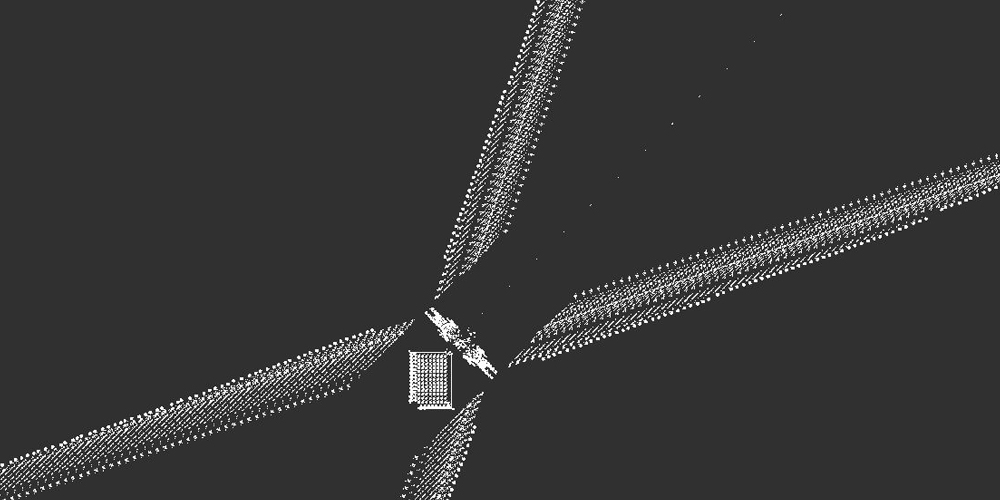
Universal Turing Machine, Initial Configuration, via Giulio Prisco
studying life
In order to investigate really complicated patterns, we need fast hardware and an algorithm for performing a stupendous amount of computation. In the 1980s, Bill Gosper discovered that memoized and canonicalized quadtrees could be used to simulate tremendously large patterns over enormous numbers of generations. He called the algorithm [hashlife], and what we have built here is a toy implementation, but it includes hashlife’s essential features.
But what does hashlife afford us? Why is it important? One practical application of hashlife is to help us understand the significance of Conway’s original proof.
The written proof is difficult for a layperson (like myself) to follow. But thanks to high-speed algorithms like hashlife, people have built actual self-replicating machines, including machines that replicate an instruction tape. You don’t need to prove it is possible when you can simply observe it replicating itself.
Equally interestingly, people have proven that anything that can be computed, can be computed in B3S23 in a remarkably easy-to-grasp format: They built Turing Machines.
The screenshot above is of a Turing Machine running in B3S23. It shows the 6,366,548,773,467,669,985,195,496,000th generation. Computations like this are only possible on commodity hardware when we can use algorithms like our memoized and canonicalized quadtrees.
From this we grasp that all computation can–in principle–be performed by remarkably simple devices.
Studying B3S23 helps us understand how much of the complexity we observe in our universe can actually arise from the interactions between very simple parts with very simple behaviour.
And B3S23 isn’t the only automaton to study. Most rule sets produce boring universes. “Average” from above tends towards empty space. Others fill their universes with chaos. But a few, like B3S23, support the creation of independent patterns that interact with each other.
In 1994, Nathan Thompson devised Highlife, described by the rules B36S23. In B3S23, a self-replicating pattern was proven to exist, but not devised until 2013 In B36S23, there are a number of trivial replicator patterns that can be used to engineer other patterns.
It’s easy to play with using our code:
const highlife = automaton({ B: [3, 6], S: [2, 3]});
And there are many others to try.
what do recursive algorithms tell us?
Our algorithm is, of course, a toy. We use strings for cells and keys. We have no way to evict squares from the cache, so on patterns with a non-trivial amount of entropy, we will quickly exhaust the space available to the JavaScript engine.
We haven’t constructed any way to advance an arbitrary number of generations, we can only advance a number of generations driven by the size of our square when doubled. These and other problems are all fixable in one way or another, and many non-trivial implementations have been written.
But the existence of an algorithm that runs in logarithmic time tells us that many things that seem impractical, can actually be implemented if we just find the right representation. When Conway and his students were simulating life by hand using a go board and coloured stones, nobody thought that one day you could buy a machine in a retail store that could run a Turing Machine or self-replicating pattern in a few minutes.
Breakthroughs like hashlife are more than just “optimizations,” even though thats the word used in this very essays. For problems suited to their domain, some algorithms are so much faster that they fundamentally change the way we approach solving problems.
We can and should take this thinking outside of algorithms and mathematical proofs. So many of the things we take for granted today are artefacts of constraints that no longer exist and/or can be removed if we put our minds to it. Out programming languages, our frameworks, our development processes, all of these things are driven by choices that were made when computation cycles were expensive and communication was slow.
We can and should ask ourselves what software would look like if it was many, many, many orders of magnitude faster. We can and should ask ourselves how our tools and the things we create with them would be deeply and fundamentally changed.
And then we should make it happen.
End, © 2011 Brownpau, some rights reserved
appendix: memoized and canonicalized quad trees
function mapWith (fn) {
  return (mappable) => mappable.map(fn);
}

function multirec({ indivisible, value, divide, combine }) {
  return function myself (input) {
    if (indivisible(input)) {
      return value(input);
    } else {
      const parts = divide(input);
      const solutions = mapWith(myself)(parts);

      return combine(solutions);
    }
  }
}

const memoized = (fn, keymaker = JSON.stringify) => {
    const lookupTable = Object.create(null);

    return function (...args) {
      const key = keymaker.call(this, args);

      return lookupTable[key] || (lookupTable[key] = fn.apply(this, args));
    }
  };

function memoizedMultirec({ indivisible, value, divide, combine, key }) {
  const myself = memoized((input) => {
    if (indivisible(input)) {
      return value(input);
    } else {
      const parts = divide(input);
      const solutions = mapWith(myself)(parts);

      return combine(solutions);
    }
  }, key);

  return myself;
}

const isOneByOneArray = (something) =>
  Array.isArray(something) && something.length === 1 &&
  Array.isArray(something[0]) && something[0].length === 1;

const contentsOfOneByOneArray = (array) => array[0][0];

const firstHalf = (array) => array.slice(0, array.length / 2);
const secondHalf = (array) => array.slice(array.length / 2);

const divideSquareIntoRegions = (square) => {
    const upperHalf = firstHalf(square);
    const lowerHalf = secondHalf(square);

    const upperLeft = upperHalf.map(firstHalf);
    const upperRight = upperHalf.map(secondHalf);
    const lowerRight = lowerHalf.map(secondHalf);
    const lowerLeft= lowerHalf.map(firstHalf);

    return [upperLeft, upperRight, lowerRight, lowerLeft];
  };

const KEY = Symbol('key');

const simpleKey = (something) =>
  isString(something)
  ? something
  : something[KEY];

const compositeKey = (...regions) => regions.map(simpleKey).join('');

const quadtree = memoized(
    (ul, ur, lr, ll) => ({ ul, ur, lr, ll, [KEY]: compositeKey(ul, ur, lr, ll) }),
    compositeKey
  );

const regionsToQuadTree = ([ul, ur, lr, ll]) =>
  quadtree(ul, ur, lr, ll);

const arrayToQuadTree = multirec({
    indivisible: isOneByOneArray,
    value: contentsOfOneByOneArray,
    divide: divideSquareIntoRegions,
    combine: regionsToQuadTree
  });

const isString = (something) => typeof something === 'string';

const itself = (something) => something;

const quadTreeToRegions = (qt) =>
  [qt.ul, qt.ur, qt.lr, qt.ll];

const regionsToRotatedQuadTree = ([ur, lr, ll, ul]) =>
  quadtree(ul, ur, lr, ll);

const memoizedRotateQuadTree = memoizedMultirec({
      indivisible : isString,
      value : itself,
      divide: quadTreeToRegions,
      combine: regionsToRotatedQuadTree,
      key: simpleKey
  });
appendix: naïve quad trees and coloured quad trees
function mapWith (fn) {
  return (mappable) => mappable.map(fn);
}

function multirec({ indivisible, value, divide, combine }) {
  return function myself (input) {
    if (indivisible(input)) {
      return value(input);
    } else {
      const parts = divide(input);
      const solutions = mapWith(myself)(parts);

      return combine(solutions);
    }
  }
}

const isOneByOneArray = (something) =>
  Array.isArray(something) && something.length === 1 &&
  Array.isArray(something[0]) && something[0].length === 1;

const contentsOfOneByOneArray = (array) => array[0][0];

const firstHalf = (array) => array.slice(0, array.length / 2);
const secondHalf = (array) => array.slice(array.length / 2);

const divideSquareIntoRegions = (square) => {
    const upperHalf = firstHalf(square);
    const lowerHalf = secondHalf(square);

    const upperLeft = upperHalf.map(firstHalf);
    const upperRight = upperHalf.map(secondHalf);
    const lowerRight = lowerHalf.map(secondHalf);
    const lowerLeft= lowerHalf.map(firstHalf);

    return [upperLeft, upperRight, lowerRight, lowerLeft];
  };

const regionsToQuadTree = ([ul, ur, lr, ll]) =>
  ({ ul, ur, lr, ll });

const arrayToQuadTree = multirec({
    indivisible: isOneByOneArray,
    value: contentsOfOneByOneArray,
    divide: divideSquareIntoRegions,
    combine: regionsToQuadTree
  });

const isString = (something) => typeof something === 'string';

const itself = (something) => something;

const quadTreeToRegions = (qt) =>
  [qt.ul, qt.ur, qt.lr, qt.ll];

const regionsToRotatedQuadTree = ([ur, lr, ll, ul]) =>
  ({ ul, ur, lr, ll });

const rotateQuadTree = multirec({
    indivisible : isString,
    value : itself,
    divide: quadTreeToRegions,
    combine: regionsToRotatedQuadTree
  });

const combinedColour = (...elements) =>
  elements.reduce((acc, element => acc === element ? element : '❓'))

const regionsToColouredQuadTree = ([ul, ur, lr, ll]) => ({
    ul, ur, lr, ll, colour: combinedColour(ul, ur, lr, ll)
  });

const arrayToColouredQuadTree = multirec({
  indivisible: isOneByOneArray,
  value: contentsOfOneByOneArray,
  divide: divideSquareIntoRegions,
  combine: regionsToColouredQuadTree
});

const colour = (something) => {
    if (something.colour != null) {
      return something.colour;
    } else if (something === '⚪️') {
      return '⚪️';
    } else if (something === '⚫️') {
      return '⚫️';
    } else {
      throw "Can't get the colour of this thing";
    }
  };

const isEntirelyColoured = (something) =>
  colour(something) !== '❓';

const rotateColouredQuadTree = multirec({
    indivisible : isEntirelyColoured,
    value : itself,
    divide: quadTreeToRegions,
    combine: regionsToRotatedQuadTree
  });
afterward
There is more to read about multirec in the previous essays, From Higher-Order Functions to Libraries And Frameworks and Why recursive data structures?.
Have an observation? Spot an error? You can open an issue, discuss the post on hacker news or even edit this page yourself.
notes
-
Actually, there is another, far more delightful way to memoize recursive functions: You can read about it in Fixed-point combinators in JavaScript: Memoizing recursive functions. ↩