
Note well: This is an unfinished work-in-progress.
Turing Machines and Tooling, Part I
Much is made of “functional” programming in JavaScript. People get very excited talking about how to manage, minimize, or even eliminate mutation and state. But what if, instead of trying to avoid state and mutation, we embrace it? What if we “turn mutation up to eleven?”
We know the rough answer without even trying. We’d need a lot of tooling to manage our programs. Which is interesting in its own right, because we might learn a lot about tools for writing software.
So with that in mind, let’s begin at the beginning.
turing machines
In 1936, Alan Turing invented what we now call the Turing Machine in his honour. He called it an “a-machine,” or “automatic machine.”1 Turing machines are mathematical models of computation reduced to an almost absurd simplicity. Computer scientists like to work with very simple models of computation, because that allows them to prove important things about computability in general.
Turing had worked with other model of computation. For example, he was facile with combinatorial logic, and discovered what is now called the Turing Combinator: (λx. λy. (y (x x y))) (λx. λy. (y (x x y))).
Turing’s “a-machine” model of computation differed greatly from combinatorial logic and the other historically significant model, the lambda calculus. Where combinatorial logic and the lambda calculus both modelled computation as expressions without side-effects, mutation, or state, his “a-machine” modelled computation as side-effects, mutation, and state without expressions.
This new model allowed him to prove some very important results about computability, and as we’ll see, it inspired John von Neumann’s designed for the stored-program computer, the architecture we use to this day.

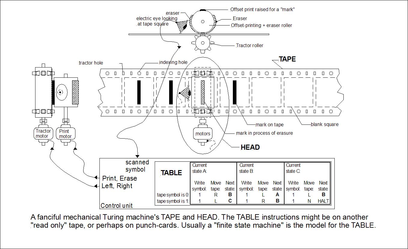
So what was this “a-machine” of his? Well, he never actually built one. It was a thought experiment. He imagined an infinite paper tape. In his model, the tape had a beginning, but no end. (If you have heard Turing machines described as operating on a tape that stretches to infinity in both directions, be patient, we’ll explain the difference later.)
The tape is divided into cells, each of which is either empty/blank, or contains a mark.
Moving along this tape is the a-machine (or equivalently, moving the tape through the a-machine). The machine is, at any one time, positioned over exactly one cell. The machine is capable of reading the mark in a cell, writing a mark into a cell, and moving once cell in either direction.
Turing machines have a finite and predetermined set of states that they can be in. One state is marked as the start state, and when a Turing machine begins to operate it begins in that state, and begins positioned over the first cell of the tape. While operating, a Turing machine always has a current state.
When a Turing machine is started, and continuously thereafter, it reads the contents of the cell in its position, and depending on the current state of the machine, it:
- Writes a mark, moves left, or moves right, and;
- Either changes to a different state, or remains in the same state.
A Turing machine is defined such that given the same mark in the current cell, and the same state, it always performed the same action. Turing machines are deterministic.
The machine continues to operate until one of two things happens:
- It moves off the left edge of the tape, or;
- There is no defined behaviour for its current state and the symbol in the current cell.
If either of these things happens, the machine halts.
our first turing machine
Given the definition above, we can write a Turing machine emulator. We will represent the tape as an array. The 0th element will be the start of the tape. As the machine moves to the right, if it moves past the end of our array, we will append another element. Thus, the tape appears to be infinite (or as large as the implementation of arrays allows). Marks on the tape will be represented by numbers and strings. By default, 0 will represent an empty cell (although anything will do).
Turing used tables to represent the definitions for his a-machines. We’ll use an array of arrays, as the “description” of the Turing machine. Each element of the description will be an array containing:
- The current state, represented as a string.
- The current mark, represented as a string or number.
- The next state for the machine (it can be the same as the current state).
- An action to perform (a mark to write, or instructions to move left, or move right).
Naturally, we’ll write it as a function that takes a description and a tape as input, and—if the emulated machine halts—outputs the state of the tape.
const ERASE = 0;
const PRINT = 1;
const LEFT = 2;
const RIGHT = 3;

function aMachine({ description, tape: _tape = [0] }) {
  const tape = Array.from(_tape);

  let tapeIndex = 0;
  let currentState = description[0][0];

  while (true) {
    const currentMark = tape[tapeIndex];

    if (![0, 1].includes(currentMark)) {
      // illegal mark on tape
      return tape;
    }

    const rule = description.find(([state, mark]) => state === currentState && mark === currentMark);

    if (rule == null) {
      // no defined behaviour for this state and mark
      return tape;
    }

    const [_, __, nextState, action] = rule;

    if (action === LEFT) {
      --tapeIndex;
      if (tapeIndex < 0) {
        // moved off the left edge of the tape
        return tape;
      }
    } else if (action === RIGHT) {
      ++tapeIndex;
      if (tape[tapeIndex] == null) tape[tapeIndex] = 0;
    } else if ([ERASE, PRINT].includes(action)) {
      tape[tapeIndex] = action;
    } else {
      // illegal action
      return tape;
    }

    currentState = nextState;
  }
}
Our “a-machine” has a “vocabulary” of 0 and 1: These are the only marks allowed on the tape. If it encounters another mark, it halts. These are also the only marks it is allowed to put on the tape, via the ERASE and PRINT actions. It selects as the start state the state of the first instruction.
Any finite number of states are permitted. Here is a program that prints a 1 in the first position of the tape, and then halts:
const description = [
  ['start', 0, 'halt', PRINT]
];

aMachine({ description })
  //=> [1]
It starts in state start because it is the first (and only) instruction. It is for our convenience that the state is called “start.” The instruction matches a 0, and the action is to PRINT a 1. So given a blank tape, that’s what it does. It then transitions to the halt state.
What happens next? Well, it is in the halt state. It is positioned over a 1. But there is no instruction matching a state of halt and a mark of 1 (actually, there is no instruction matching a state of halt at all). So it halts.
Given a tape that already has a 1 in the first position, it halts without doing anything, because there is no instruction matching a state of start and a 1. We can add one to our program:
const description = [
  ['start', 0, 'halt', PRINT],
  ['start', 1, 'halt', ERASE]
];

aMachine({ description, tape: [0] })
  //=> [1]

aMachine({ description, tape: [1] })
  //=> [0]
We’ve written a “not” function. Let’s write another. Let’s say that we have a number on the tape, represented as a string of 1s. So the number zero is an empty tape, the number one would be represented as [1], two as [1, 1], three as [1, 1, 1] and so forth.
Here’s a program that adds one to a number:
const description = [
  ['start', 0, 'halt', PRINT],
  ['start', 1, 'start', RIGHT]
];

aMachine({ description, tape: [0] })
  //=> [1]

aMachine({ description, tape: [1] })
  //=> [1, 1]

aMachine({ description, tape: [1, 1] })
  //=> [1, 1, 1]
If it encounters a 0, it prints a mark and halts. If it encounters a 1, it moves right and remains in the same state. Thus, it moves right over any 1s it finds, until it reaches the end, at which point it writes a 1 and halts.
All of our machines so far have one “real” state, start, and one deliberately “undefined” state, halt. We can write programs with more than one state. This one prints a 1 in the third position on the tape:
const description = [
  ['start', 0, 'one', RIGHT],
  ['start', 1, 'one', RIGHT],
  ['one', 0, 'two', RIGHT],
  ['one', 1, 'two', RIGHT],
  ['two', 0, 'halt', PRINT]
];

aMachine({ description })
  //=> [0, 0, 1]
It has three different states (plus “halt”).
expressiveness and power
Our “a-machine” is very simple. It does allow for as many states as we like, but only two symbols. Each instruction can only print, erase, or move. Despite its simplicity, Alan Turing proved that anything that can be computed, can be computed by an a-machine. This is not an essay about computer science, so we won’t concern ourselves with the formal proof.
Instead, we will follow the path of demonstrating why an a-machine is much more powerful than it may appear. Our method will be this:
First, we designate the a-machine as being the simplest possible type of Turing machine. Meaning, it has the least possible “expressiveness” of descriptions. Next, we think of a Turing machine that is more expressive than an a-machine. How do we demonstrate that despite being more expressive, the new machine is no more powerful than an a-machine?
We show how to transform any input for our more expressive machine into input for an a-machine. And we show how to transform the output of our a-machine into the output for our more powerful machine. If we can do both of these things, we can grasp that the two machines have equivalent power. Meaning, that both can compute exactly the same things.
the sequence-machine
Here is a Turing machine that is undeniably more expressive than an a-machine. Its principle advantage is that it permits any sequence of actions to be associated with a single instruction:
function sequenceMachine({ description, tape: _tape = [0] }) {
  const tape = Array.from(_tape);

  let tapeIndex = 0;
  let currentState = description[0][0];

  while (true) {

    const currentMark = tape[tapeIndex];

    if (![0, 1].includes(currentMark)) {
      // illegal mark on tape
      return tape;
    }

    const rule = description.find(([state, mark]) => state === currentState && mark === currentMark);

    if (rule == null) {
      // no defined behaviour for this state and mark
      return tape;
    }

    const [_, __, nextState, ...actions] = rule;

    for (const action of actions) {
      if (action === LEFT) {
        --tapeIndex;
        if (tapeIndex < 0) {
          // moved off the left edge of the tape
          return tape;
        }
      } else if (action === RIGHT) {
        ++tapeIndex;
        if (tape[tapeIndex] == null) tape[tapeIndex] = 0;
      } else if ([ERASE, PRINT].includes(action)) {
        tape[tapeIndex] = action;
      } else {
        // illegal action
        return tape;
      }
    }

    currentState = nextState;
  }
}
It runs all the programs written for an a-machine:
const description = [
  ['start', 0, 'one', RIGHT],
  ['start', 1, 'one', RIGHT],
  ['one', 0, 'two', RIGHT],
  ['one', 1, 'two', RIGHT],
  ['two', 0, 'halt', PRINT]
];

sequenceMachine({ description })
  //=> [0, 0, 1]
But it can also run a new kind of program that an a-machine cannot run:
const description = [
  ['start', 0, 'halt', RIGHT, RIGHT, PRINT],
  ['start', 1, 'halt', RIGHT, RIGHT, PRINT]
];

sequenceMachine({ description })
  //=> [0, 0, 1]
This is a much more convenient way to run programs. Is it more powerful? No.
demonstrating that a sequence-machine is no more powerful than an a-machine
We started with a program for an a-machine that looked like this:
const description = [
  ['start', 0, 'one', RIGHT],
  ['start', 1, 'one', RIGHT],
  ['one', 0, 'two', RIGHT],
  ['one', 1, 'two', RIGHT],
  ['two', 0, 'halt', PRINT]
];
And we transformed it into a program for a sequence-machine that looked like this:
const description = [
  ['start', 0, 'halt', RIGHT, RIGHT, PRINT],
  ['start', 1, 'halt', RIGHT, RIGHT, PRINT]
];
To demonstrate that a sequence-machine is no more powerful than an a-machine, we will do the reverse: We will show that we can transform any description of a sequence-machine into a description of an a-machine that produces the same result.
Here is our demonstration written in JavaScript:
// prologue: some handy functions

const flatMap = (arr, lambda) => {
  const inLen = arr.length;
  const mapped = new Array(inLen);

  let outLen = 0;

  arr.forEach((e, i) => {
    const these = lambda(e);

    mapped[i] = these;
    outLen = outLen + these.length;
  });

  const out = new Array(outLen);

  let outIndex = 0;
  for (const these of mapped) {
    for (const e of these) {
      out[outIndex++] = e;
    }
  }

  return out;
};

const gensym = (()=> {
  let n = 1;

  return (prefix = 'G') => `${prefix}-${n++}`;
})();

const times = n =>
  Array.from({ length: n }, (_, i) => i);

// flatten, transform any description for a sequence-machine into
// a description for an a-machine

const flatten = ({ description: _description, tape }) => {
  const description = flatMap(_description, ([currentState, currentMark, nextState, ...instructions]) => {
    if (instructions.length === 0) {
      // pathological case
      return [];
    } else {
      const len = instructions.length;
      const nextStates = [];

      let destinationState = nextState;

      times(len).forEach( () => {
        nextStates.unshift(destinationState);
        const match = destinationState.match(/^\*(.*)-\d+$/)

        if (match) {
          destinationState = gensym(`*${match[1]}`);
        } else destinationState = gensym(`*${destinationState}`);
      });

      const currentStates = nextStates.slice(0, len - 1);
      currentStates.unshift(currentState);

      let possibleMarks = [currentMark];

      const compiled = flatMap(times(len), i => {
        const instruction = instructions[i];

        const mappedInstructions = possibleMarks.map(
          mark => [currentStates[i], mark, nextStates[i], instruction]
        );

        if ([LEFT, RIGHT].includes(instruction)) {
          possibleMarks = [0, 1];
        } else if ([ERASE, PRINT].includes(instruction)) {
          possibleMarks = [instruction.mark];
        }

        return mappedInstructions;
      });

      return compiled;
    }
  });

  return { description, tape };
}
We can “flatten” any description for a sequence-machine into a description for an a-machine:
const description = [
  ['start', 0, 'halt', RIGHT, RIGHT, PRINT],
  ['start', 1, 'halt', RIGHT, RIGHT, PRINT]
];

flatten({ description, tape: [0] })
  //=>
    {
      description: [
        ["start", 0, "*halt-2", 3],
        ["*halt-2", 0, "*halt-1", 3],
        ["*halt-2", 1, "*halt-1", 3],
        ["*halt-1", 0, "halt", 1],
        ["*halt-1", 1, "halt", 1],
        ["start", 1, "*halt-5", 3],
        ["*halt-5", 0, "*halt-4", 3],
        ["*halt-5", 1, "*halt-4", 3],
        ["*halt-4", 0, "halt", 1],
        ["*halt-4", 1, "halt", 1]
      ],
      tape: [0]
    }
Although it has a few moving parts, what it does at its simplest is turn any instruction with more than one action into a series of instructions, one per action. To chain them together, it creates “synthetic” states like *halt-2. It also tries to make moving robust to account for any marks the machine may encounter.
If we run our flattened description, we see it produces the same output:
aMachine(flatten({ description, tape: [0]}))
  //=> [0, 0, 1]
Now, it’s not exactly the same program that we originally wrote. Our program had fewer states, because we optimized for having a single state for each cell we moved over. The flatten function is very conservative. But it will produce a description for an a-machine that performs the same computation, so we can convince ourselves informally that anything a sequence-machine can compute, so can an a-machine, because any member of the set of all possible sequence-machine descriptions maps to at least one member of the set of all possible a-machines.
from computer science to tooling
That is an interesting result in Computer Science, and we will follow the same reasoning to work with other types of Turing machines. But our focus is on something else, tooling. Did you notice that flatten is a tool? It’s a compiler, and it is no different in principle than something like ClojureScript or Babel. It compiles a program written in a more-expressive language into one written in a less-expressive language.
And that is very interesting.
We earlier defined what we meant by two machines having equivalent power. Let’s quickly say what we mean about being “more expressive.” There are a few different concepts in play, but one of the most obvious is that for a given computation, the description that contains less accidental complexity.
So when looking at this description of an a-machine:
const description = [
  ['start', 0, 'one', RIGHT],
  ['start', 1, 'one', RIGHT],
  ['one', 0, 'two', RIGHT],
  ['one', 1, 'two', RIGHT],
  ['two', 0, 'halt', PRINT]
];
We can take the position that the states start and halt are “essential” complexity, but the states one and two are artefacts of the solution domain, they’re how we implement moving right twice. So they are “accidental” complexity. This description of a sequence-machine:
const description = [
  ['start', 0, 'halt', RIGHT, RIGHT, PRINT],
  ['start', 1, 'halt', RIGHT, RIGHT, PRINT]
];
Appears to eliminate the one and two states. Naturally, we know that it actually creates at much actual complexity as the original hand-coded description:
[
  ["start", 0, "*halt-2", 3],
  ["*halt-2", 0, "*halt-1", 3],
  ["*halt-2", 1, "*halt-1", 3],
  ["*halt-1", 0, "halt", 1],
  ["*halt-1", 1, "halt", 1],
  ["start", 1, "*halt-5", 3],
  ["*halt-5", 0, "*halt-4", 3],
  ["*halt-5", 1, "*halt-4", 3],
  ["*halt-4", 0, "halt", 1],
  ["*halt-4", 1, "halt", 1]
]
But as programmers, we don’t appear to see that complexity, so it feels like it has been eliminated.
comparing compilers to interpreters
We actually have two different implementations of the “sequence-machine.” The first one we look at is basically an interpreter that understands and executes instructions with multiple actions. The second one we looked at compiles a sequence-machine description into an a-machine description.
We have analogues for this in the “real world” as well. We have tools like Babel that translate various cutting-edge dialects of JavaScript into a more basic flavour of JavaScript. But we also have browsers like Safari and Chrome gradually incorporating more expressive flavours of JavaScript into their underlying engines.
What are the relative tradeoffs of the two approaches? In broad terms, it often comes down to how we want to manage the complexity we’re trying to hide. We are going to implement more expressive Turing machines over the coming posts. With each one, we have to manage more and more complexity.
When we push that complexity into the interpreter (or “engine”), we often find the engine getting a little more complicated. In our very simple example, both the “a-machine” and the “sequence-machine” have while loops to iterate step-by-step through the instructions as the machine operates. But to handle multiple actions within a single instruction, the “sequence-machine” adds a for loop within the while loop.
Whereas, the “flatten” complier we wrote obviously doesn’t add anything to the “a-machine,” it translates programs for the sequence-machine into programs for the a-machine and then runs them on the unmodified a-machine code. That being said, compilers often appear more complicated than the code they add to interpreters. “flatten” certainly has lots more code than the changes we made to transform an a-machine into a sequence-machine.
so why build compilers?
The compiler solution has one very powerful advantage over the interpreter, despite its size. The compiler absolutely and positively separates the concern of handling sequences from the concern of interpreting instructions for an a-machine. If we want to know what we have to do to handle sequences, all the code we need to read is in “flatten.”
Whereas, in the sequence-machine, the code handling sequences is embedded. It’s not factored out into a separate function or module. As we add more features to interpreters, our interpreters tend to grow higgledy-piggledy, with the considerations for each feature coupled to every other feature’s code.
We can and should work to separate these concerns, but that does not come “for free.” When writing interpreters, the default or easiest path is for them to grow in complexity. But what about compilers?
As we add new functionality, if we add it to “flatten” to make a super-compiler, we have the same problem. But compilers don’t have to grow this way by default.
In Part II, we are going to add more functionality, and look at how we can pipeline compilers, a pattern that naturally separates and modularizes concerns.
notes
-
In this essay, we will call his model an “a-machine” when discussing his work in historical context, but call the machines we build in the present tense, “Turing machines.” ↩